TUTORIAL 9
9.1. Introduction
You have already read about waveforms and traces. Now you will read about how to make traces from waveforms. Recall that a trace consists of a group of frames. Waveforms can be broken up into frames based on any trigger you chose. A trigger is any point at which you want to start a frame. In the Analysis program, triggers must be spikes. However, a spike need not be an actual action potential. It can be anything (almost) such as a marker pulse or even a step cycle.
The usefulness of this is that, once you have frames, these can be tagged (labeled if you want) with a number code and all trace analyses can be performed on either all the frames (by selecting all tags) or on a subset of the traces (by selecting one or a few tags).
This tutorial will uses an example (explained in Section 9.1) to illustrate the general procedure of reframing. Whatever you want to base your reframing on, the idea is exactly the same. The only change is what is used as a trigger. Often it will be a stimulus marker in which case the marker will be defined as a spike and then used as the trigger.
Note that throughout this tutorial, underlined characters indicate variables and italics indicate commands or names that are used in Analysis.
9.1 Reframing as an indirect way to tag cycles
Reframing can also be used as an indirect way to tag cycles. Suppose you have defined cycles and that you want to label them as being either a control cycle or a stimulated cycle. Strictly speaking there is no direct way to do this in Analysis. The indirect way to do this is to cheat and set spikes but using cycles. Said differently, you pretend that a cycle burst is a spike. Once you have set these “spikes” using a reliable ENG, you can reframe the waveforms of your choice and thus create traces. If you set your average window and delay properly you can get the whole cycle included in the trace and you can also center it any way you want.
There is a hitch though with using cycles to reframe. What if you do not have a reliable ENG? This was my case since I was looking at deletions which are missing bursts of activity. During the deletions, either the burst is gone entirely or it is greatly reduced. Since the set spikes allows only one set of parameters to be used for threshold, hysteresis, and discriminator, it works best when all the bursts are of similar amplitude. That didn’t apply to my data set. The way around this was to use set spike train option. The goal is to set a spike train of one spike for each cycle. This can be done either automatically or manually which allows for adding pairs (hence spike trains) anywhere you click. The procedure first requires that you set spikes although and afterwards you can add spike trains where you have missed.
9.2. Selecting the waveforms and range of interest
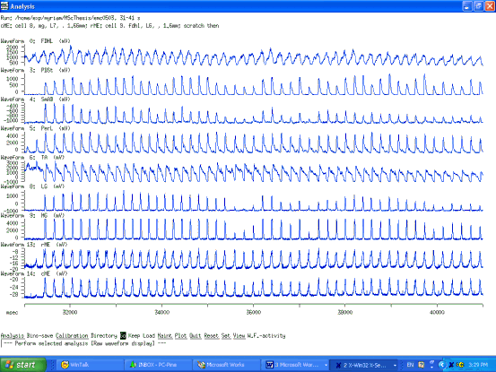
The first step is the selection of the waveforms and range of interest within the data file. All waveforms can be inspected with the analysis/raw-waveform/go command. Then, specific ones can be listed and displayed using the set/W.F.-disp./list/1-4 enter/quit/quit/go command. The syntax for entering waveforms is as follows. 1:4 will display waveforms 1,2,3, and 4 whereas 1,4 will display waveforms 1 and 4 only. A space between numbers acts like a comma and a dash acts like a colon. The range to be displayed and analysed can be set say, from 30 seconds to 60 seconds, with the command set/range/start/30s enter/end60s enter/go/.
Figure 1 Selecting the range and waveforms of interest

9.3. Setting the trigger for the frames
First a reliable and clean ENG must be chosen. It must be reliable in the sense that it must have a burst in every cycle (i.e. no deletion) however small a burst, otherwise we won’t be able to reframe that particular cycle and this would defeat the purpose! The ENG must be clean in the sense that the burst should be as smooth as possible since this will make setting the spike parameters much easier. But we can make do with less than ideal conditions. A third point is this: what is the difference between setting spikes and setting spike trains and how can we use the spike trains setting to our advantage?
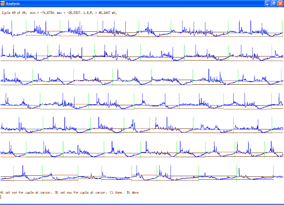
There are two things which we need to do. Cut the waveforms into frames, one for each cycle, so that we can tag these frames as belonging either to the control group or the deletion group so we can perform averages of each group. This is performed using the reframe command which takes spikes as triggers of the frames and cuts desired waveforms producing a corresponding trace for it. The other thing we need to do is measure the LDP of each cycle. This could be done on the traces manually using QM and writing down the result but this is tedious and not very reproducible. We want to take advantage of the analysis option of the graph of LDPs vs start time of the cycle. To do this we need to set the cycles. How can we make sure that these cycles have the same borders as the frames we created? By using the set/cycles/trains command which uses spike trains as the borders of cycles. The first spike train will be the beginning of the first cycle, the second spike will be the end of the first cycle and the beginning of the second cycle and so on. Thus, for 50 spike trains one will have 49 cycles.
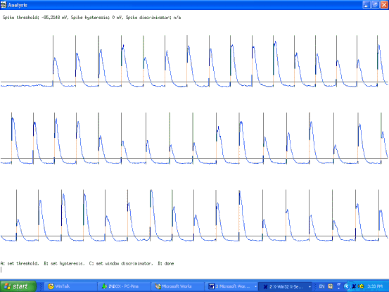
To set spike trains one must first set spikes using W.F. – activity 3/set/spikes/visually/ and use the mouse to set the threshold, hysteresis, and discriminator. Then after clicking done choose trains/automatic/done. Select the minimum gap between spike trains with gap 0.2 . Then perform manual spike train selection with the manual command, This will allow you to simply add pairs of cursors where new trains should be inserted, in much the same way that cycles can be specified manually. It is important that the spike trains and the spikes be identical since the frames are triggered fronm the spikes whereas the cycles are determined from the spike trains.
Figure 2 Setting spikes on the reliable ENG chosen
9.4. Displaying traces in Analysis
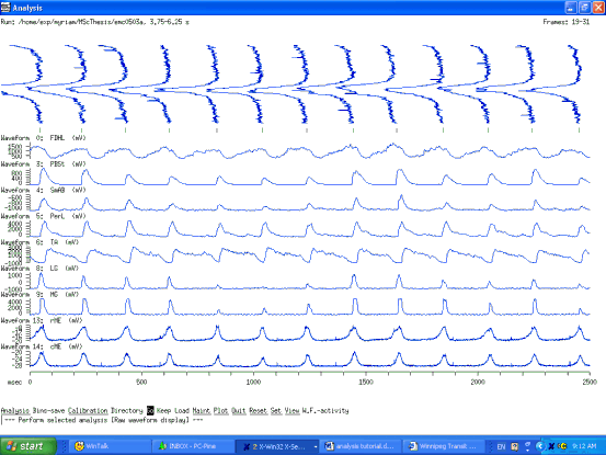
To display the frames created by the reframe command one must first modify the display window to allow frames from one trace to be displayed at the top of the waveforms. This is done using the set/disp-opt/waveform/mark-frames/yes command. The choice of the trace to be displayed is done with the command set/levels/trace/number 13 .
Figure 3 How to display the traces generated by the reframe command
9.5. Displaying and handling traces in Frameselect
Traces can be deleted and in this way removed from the analysis. This could be done for instance if a certain trace contains an artifact from a stimulus or a cal pulse which we were not supposed to have on and so on. Trace deletion is done in Frame Select and is reversible. To invoke Frame Select from Analysis choose Maintenance/Select-Frames. A new window of the Frmsel program will then open and show the info displayed in Figure 1. It shows how many traces there are in the run, how many frames they are made of and other such information.
Figure 4 Initial window in Frame Select
To display all the traces so they can be viewed and the appropriate ones deleted one needs to set a few parameters:
• interpolate/yes This is so the traces do not show up as almost invisible dotted lines.
• trace/3 enter This is to choose the trace to be displayed.
• rows-cols-scale /10 enter 4 enter 0 enter. I find that a 10 by 4 array of traces usually gives me a very good view for the purpose of deleting traces. 0 indicates that autoscaling is in effect so traces are not all magnified in the same way. The magnification factor is displayed so you can judge what is bigger than what. Once you have a feel for it you can display everything at the same scaling factor especially if they don’t vary too much. In this example in Figure 5, most traces were at x16 and a few at x32. Therefore it was suitable to display them all at x16.
Figure 5 Display of traces in Frame Select
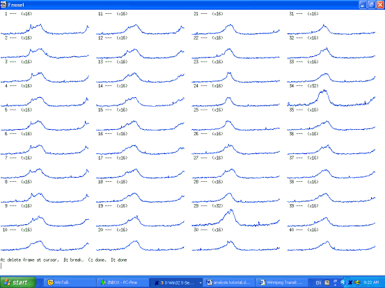
Figure 5 Display of traces in Frame Select with some traces deleted (those with a big X on them)
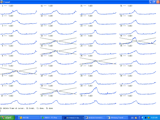
To delete traces, simply click on them and an X will appear on the deleted traces. To tag the frames with say number 2, use the number-tags command in Frmsel. This command first prompts you for the tag you want to give to a particular set of frames. The tag can have a value from 0 to 4095 and the value chosen is arbitrary. Then you need to enter which frames should be given that particular tag. You can enter a list using the same convention as when entering a waveform list in Analysis. In my case I wanted to tag all control frames with 1 and a few deletions with 2. Then it is easiest to do number-tags/1 /all followed by number-tags/2 /list of frames with deletions . This avoids entering a long list of control frames to be tagged. Tags are overwritten by new entries. With the number-tags command you can also enter a sequence of tags to be applied repeatedly to the frames.
9.6. Performing analyses on a subset of the frames from a trace
Frames can be analysed separately according to their tag. First choose the tag to be analysed with the command set/tags/2 . set/tags/all incorporates all frames (except those deleted of course) in the analysis regardless of their tag.
Figure 7 Performing the averages of the traces bearing a certain tag
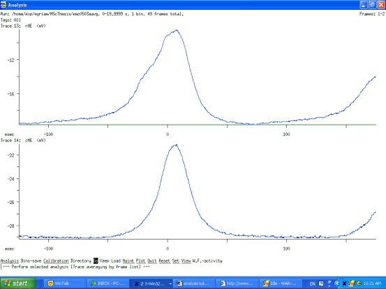
Once the averages are performed for each tag, they can be saved into new run files using the bins-save command. If the set/avg/preview/ command is set to yes , then all the frames to be averaged are displayed first. When that is the case, one can save either the average or the ensemble of frames included in this average. To save the average itself answer no N to the save raw (previewed data) instead of average? that comes up after the bins-save command. To save the frames answer yes Y to the same question.
9.7. Appending averages with the Appendrun command
If you perform averages for different groups, these can be appended so they are part of the same run file and can be viewed simultaneously as in Figure 8. This is performed from the command line with the appendrun command. The syntax is appendrun file1 file2. This means that file2 will be appended in file1 which will be overwritten in the process. Averages from file1 will become the first frames in the traces and averages in file2 will become the second frames and so on. Trace numbers will remain the same.
Figure 8 Looking at the two separate averages in Qm after they are appended (Frame 1 is the average of control cycles, Frame 2 is the average of deletion cycles.)
9.8. Displaying frames with the Raster program
The frames that were included in an average can be looked at individually using the Raster program as shown in Figure 9. To set which trace is looked at choose File/emc0503/trace number/all all indicates that all frames should be displayed. ( I think that still excludes deleted frames although.) . interpolate/Y should be set. Also, one can change the appearance of the display by setting the x and y increments to different values. Having both to be nonzero displays them diagonally. In Figure 9, X-incr/10 and Y-incr/10. If both were 0 then all traces would be superimposed.
Figure 9. Raster plot of all the traces that were included in the average. This is produced by setting yes to preview and by choosing the preview t obe saved when doing a bins-save.
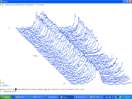
Figure 10 Cycle durations can be displayed under the waveform (set/w/cyle-length)
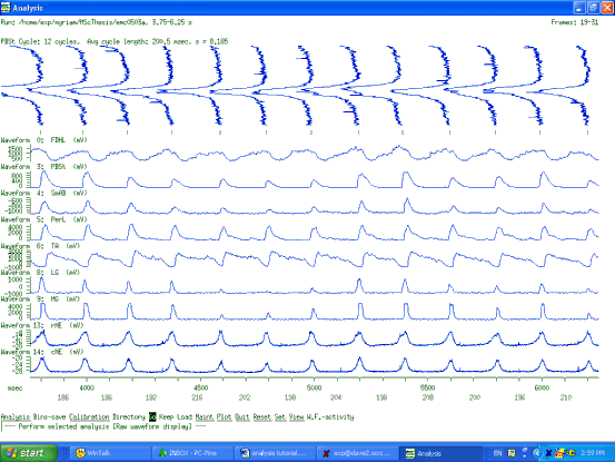
Figure 11 And the cycle markers for the ON and OFF phases too!

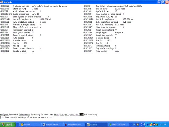
Figure 12 View required for doing a graph of LDP vs cycle duration
9.9 Subtleties about setting spikes and spike trains
Figure 13 From top to bottom discriminator, threshold, hysteresis (ie hysteresis below threshold for upgoing spikes)
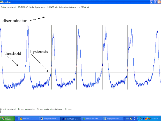
Figure 14 From top to bottom, discriminator, hysteresis, threshold (ie hysteresis above threshold for downgoing spikes)
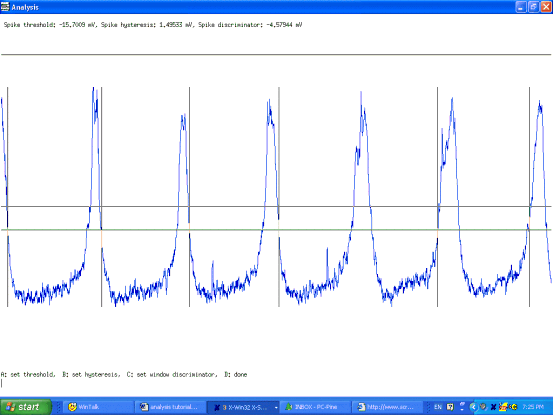
Figure 15 Setting LDP boundaries manually for graph analysis of LDP in each cycle
Syntax: dumprun runfile
Dumprun displays the contents of the run header for each named run. Each name specified as an argument may be either the name
of a frame file, or the name of a run without the .frm suffix. Several lines will be displayed for each run, starting with general
information about the run, and followed by the calibration information for each stored trace and waveform. There are options to convert
the data points in frames or traces to ASCII values and display them.
dumprun [ -f ] [ -t ] [-c n]
With the -f option, dumprun will display (dump out) the frame header for each frame, following the run header contents. With the -t , it
will dump out not only the frame headers, but also the trace data within each frame, as decimal integer values representing the raw
A/D levels recorded. This gives an ASCII text representation of the entire frame file. By default, the trace data will be presented as a
single column, one number per line. A greater number of columns can be selected with the -c option. The samples should be read
along rows rather than down the columns.
dumprun can be used to move trace data into a spreadsheet for further analysis. For example, create an average of several frames
and save it (Bins-save) as "myfile". Then use dumprun to create a new file with the data points as integers. Eg.
dumprun -t myfile > temp.prn
Now read "temp.prn" into your favourite spreadsheet as an ascii file
This command is useful to obtain the trigger times of frames.